6. Technical Notes
6.1. MLSDK for MN-Core
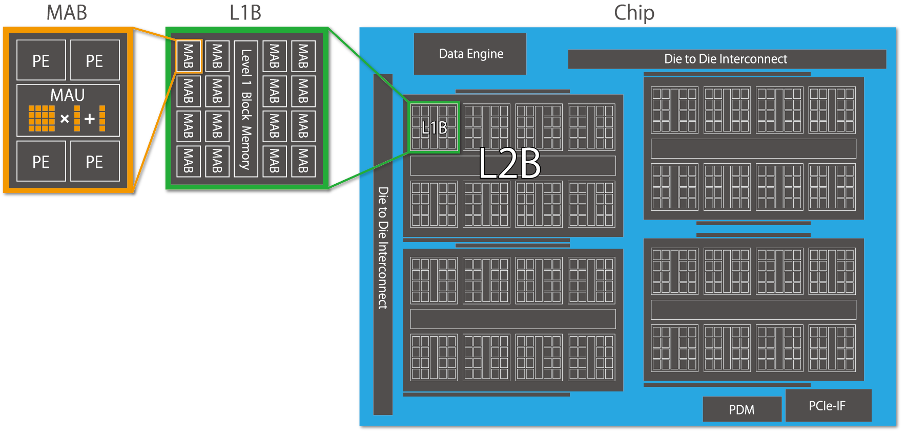
Fig. 6.1 MN-Core’s hierarchical architecture
The defining characteristic of the MN-Core series is its hierarchical structure, as illustrated in Fig. 6.1. Each Processing Element (PE) possesses its own Local Memory (LM) and General Register File (GRF), which correspond to the leaf nodes of a tree-like memory hierarchy. Notably, the LM combines the advantages of high-speed SRAM access from the PE with substantial total capacity, enabling minimal DRAM access and effectively improving the overall B/F ratio. However, it lacks advanced memory management features like cache memory, and all data transfers must be explicitly specified. For more detailed information about MN-Core 2 itself, please refer to mncore2_dev_manual_ja.pdf.
When using MN-Core 2 as a backend for PyTorch through the MLSDK, knowledge of assembly instructions or instruction formats is not required. However, understanding how computation graph inputs/outputs and intermediate Tensors utilize memory will enable more advanced utilization of the MLSDK. When storing each Tensor in MN-Core 2’s internal memory, the MLSDK’s graph compiler (codegen) determines the following three key aspects:
Dtype : The numerical precision of the Tensor
Location : Whether to store the Tensor in DRAM or LM
Layout : How the Tensor should be mapped to the memory hierarchy
Regarding Dtype, the basic precision is inherited from the original Tensor. However, for operations like matrix multiplication and convolutions, temporary precision reduction may be employed for faster computation. Conversely, for operations requiring high precision such as BatchNormalization, the precision is restored for accurate computation. Known as mixed precision computing, this mechanism is widely adopted in machine learning frameworks—PyTorch implements it through torch.amp —and the MLSDK maintains consistent numerical precision across the entire computation graph by managing each Dtype.
Regarding Location and Layout, these are determined based on the original Tensor’s shape and the previously set Dtype. Since computation results may be reused at multiple locations or individual computation processes may require different mappings, a structure called MNValue is prepared for each Tensor, which contains Location and Layout information. The mechanisms for determining these properties are more complex than those for Dtype, with their details explained in Location Planner and Layout Planner. Importantly, both Location and Layout settings directly impact LM consumption, each influencing the planning process. Furthermore, depending on the Tensor’s shape and the Layout that represents it, the computation may not even fit within the available LM capacity. In such cases, Time-Slice is applied, dividing the computation into multiple sequential stages.
The current codegen system considers these three factors in sequence to determine the Dtype, Location, and Layout as follows:
Dtype Planner: Determines numerical precision and roughly estimates the LM consumption for each Tensor
Location Planner (initial): Identifies Tensors—such as model parameters—that must be reliably placed in DRAM
Layout Planner: Determines Layout according to the requirements of computation nodes (MNNode), while also considering whether MNValues will be stored in DRAM or LM
Location Planner: Finalizes Location determination while also taking into account the LM consumption calculated from the Layout
Time-Slice: Applies time-division to MNValues that exceed LM capacity but must be placed in LM due to MNNode requirements
Location Planner (sliced): Adjusts Location assignments to account for the effects of time-division
After these processes determine both the computational graph (MNGraph) managed by codegen and the information about MNNode and MNValue components that construct it, the Scheduler then performs overall scheduling. While the basic computation order is determined by topological sorting of the computational graph, additional consideration must be given to the sequence in which MNValues are placed in their assigned Locations. Although MNValue Locations guarantee that MNNodes will process data assuming those placements, there may be cases where data cannot be continuously retained in LM—such as when MNValues are reused at multiple locations. In such cases, the data must be temporarily moved to DRAM, and the scheduling system determines the optimal timing for data relocation during computation.
For example, the most straightforward Scheduler implementation is always_from_dram.
This approach writes all computed MNValues back to DRAM and reads them from DRAM whenever needed.
While this scheduling method works in most scenarios, it is not optimal by any means and is primarily intended for debugging purposes.
Therefore, the MLSDK provides multiple Scheduler options tailored to different use cases, allowing users to select the most appropriate one for their requirements.
Furthermore, achieving optimal scheduling requires not only advanced Scheduler algorithms but also detailed information about each MNNode’s execution speed and memory usage. This information collection mechanism is Node Simulation, which aggregates results from compiling each MNNode under various configurations. For instance, when an MNNode exhibits trade-offs between memory usage and execution speed, by examining both optimized memory-saving configurations and those with generous memory allocation, the Scheduler can choose settings that achieve overall optimization.
After scheduling, additional configurations such as Address are set for each MNValue, and corresponding Operators are Code Emit to generate the specific assembly code. By sequentially combining these components, the final assembly and GPFNApp compilation result are produced.While the current MLSDK does not require users to understand much about the processes following scheduling, we are actively preparing the framework to enable feature expansions, such as adding support for unimplemented Operators.
Thus far, we have explained how a computational graph input to the MLSDK is compiled to produce reusable results (GPFNApp).
The GPFNApp can be loaded by the MLSDK and invoked from Python as a mlsdk.CompiledFunction, allowing users to replace the original source function with this compiled result and thereby utilize the MN-Core 2.
Due to the time-consuming nature of Node Simulation and Scheduler operations, the MLSDK is designed with GPFNApp reuse in mind, making it particularly suitable for workloads that repeatedly execute the same computations, such as training loops or batch inference.Furthermore, because the process involves mapping data to tree-like LMs as MNValues, it performs poorly with operations requiring extensive indexing. However, it generally excels at operations with high spatial locality.
6.2. MLSDK Pipeline
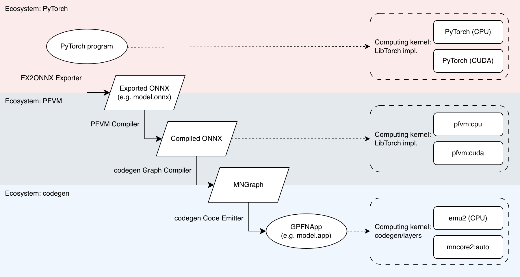
Fig. 6.2 MLSDK Pipeline and Backend Correspondence
When compiling an input (PyTorch program) for the MN-Core series, the MLSDK performs several transformations as shown in Fig. 6.2 to produce an executable binary (GPFNApp).
Here we explain the terminology used in the figure.
6.2.1. Ecosystem
The MLSDK involves multiple intermediate states before a PyTorch program can run on the MN-Core series. Each intermediate state can be output in formats like ONNX, or in some cases can be executed directly. The execution environments available are three types: PyTorch, PFVM, and codegen. We provide an overview of these.
PyTorch
This refers to the environment including torch along with related packages such as torch-vision.
The MLSDK assumes that the input program implements computation using torch.Tensor, and exports this portion as a computation graph (Exported ONNX in the figure).
The fundamental philosophy of MLSDK is that there are no restrictions on the syntax using torch.Tensor.
However, since the torch package is installed after being built with extensions specifically for MLSDK, you cannot currently use different versions within the same MLSDK environment.
For the same reason, you cannot install and use externally downloaded torch packages.
PFVM
PFVM is an environment that combines both a compiler and runtime specifically for Exported ONNX.
It works in collaboration with the FX2ONNX Exporter, which outputs computation graphs in ONNX format from PyTorch programs.
During this process, it adds missing elements from the original program—such as weight update handling—as custom ONNX operators to the Exported ONNX.
The compilation results produced by PFVM are output as structures based on ONNX (Compiled ONNX in the figure), which are then passed to the subsequent codegen stage in the pipeline.
Compiled ONNX can also be executed using PFVM’s runtime. In MLSDK, you can specify pfvm:cpu or pfvm:cuda as arguments to mlsdk.MNDevice to respectively use CPU and GPU.
In this context, each operator in the computation graph is implemented using LibTorch.
codegen
codegen is an environment that combines both a compiler and runtime specifically designed for MN-Core series processors, targeting Compiled ONNX.
The compilation process is divided into two major stages: the front-end is called the codegen Graph Compiler, and the back-end is called the codegen Code Emitter.
The codegen Graph Compiler outputs MNGraph after adding MN-Core series-specific operators and performing scheduling, including recomputation, on the Compiled ONNX.
Note that MNGraph is also a structure based on ONNX, meaning it can be output as a file in that format.
Next, the codegen Code Emitter generates assembly code for each operator in MNGraph, adds necessary execution information, and outputs GPFNApp.
During this process, the implementations of each operator are compiled and stored in the codegen/layers directory as shown.
Note
The implementations in codegen/layers are not yet included in the MN-Core SDK image and are instead bundled with the pre-built codegen libraries.
The resulting GPFNApp can then be executed on MN-Core 2 using codegen’s internal runtime (mncore2:auto), or alternatively in an emulator environment called emu2.
emu2 is a software that attempts to faithfully reproduce the specifications of MN-Core 2, enabling development and debugging even when access to actual MN-Core 2 hardware is not available.
Please be aware that since it emulates operation on a CPU, the performance will be significantly slower compared to physical hardware.
Additional Notes
We explain the advantages of using PFVM when porting code to the MN-Core series.
First, the processing performed by the PFVM Compiler involves substantial modifications to the computation graph, making it relatively difficult to verify correctness. The changes before and after this stage are comparatively easier to validate, so computation graphs are categorized into two types: PyTorch Graphs and Compiled Graphs.
Second, the implementation types of each operator can be divided into two categories: LibTorch and codegen/layers.
By making this distinction, the comparison between the different ecosystems becomes as follows:
PyTorch: Processes (PyTorch Graphs) using (LibTorch)
PFVM: Processes (Compiled Graphs) using (LibTorch)
codegen: Processes (Compiled Graphs) using (codegen/layers)
Directly proceeding from PyTorch to codegen involves changes in both graph structure and operator implementations. However, by first going through the PyTorch → PFVM → codegen sequence, you can independently verify both the graph structure and operator implementations.
Furthermore, even if codegen/layers contains no issues, any problems with the Compiled Graph would inevitably propagate to subsequent stages. Therefore, it’s more efficient to halt at the PFVM stage for verification.
For operational verification, we recommend first testing both pfvm:cpu and pfvm:cuda to confirm computation results and check whether any issues occur during the graph transformation process.
6.2.2. Pipeline Stage
PyTorch program – (FX2ONNX Exporter) -> Exported ONNX
The FX2ONNX Exporter is a mechanism that utilizes the torch.fx functionality to generate ONNX files.
This is an independent component from PFVM and codegen, with its Python implementation located at /opt/pfn/pfcomp/fx2onnx.
FX2ONNX Exporter is applied to the function object passed to mlsdk.Context.compile().
The function must conform to the Callcable[[Dict[str, Tensor]], Dict[str, Tensor]] type, and a symbolic trace is performed starting from each input/output torch.Tensor.
The resulting torch.fx.Graph contains operators compatible with LibTorch, which are then converted to ONNX operators to produce the Exported ONNX.
Note
During the tracing process, torch.Tensor objects are treated as torch._subclasses.fake_tensor.FakeTensor, meaning no actual computation is performed.
If your code contains conditional branches that check for the presence of torch.Tensor, proper tracing of these branches may not be guaranteed.
In addition to this FX2ONNX Exporter mechanism, there exists another method for converting PyTorch programs to ONNX: torch.onnx.
In the MLSDK environment, you can also use torch.onnx for ONNX export by setting the environment variable MNCORE_USE_LEGACY_ONNX_EXPORTER, though this feature is currently deprecated and support is limited.
However, it may be utilized in certain Examples provided in the MLSDK.
Example usage of torch.onnx:
$ cd /opt/pfn/pfcomp/codegen/examples/
$ MNCORE_USE_LEGACY_ONNX_EXPORTER=1 ./exec_with_env.sh python3 add.py
References:
Exported ONNX – (PFVM Compiler) -> Compiled ONNX
The PFVM Compiler takes Exported ONNX as input and performs various optimizations, ranging from basic operations like Constant Propagation and Common Subexpression Elimination to advanced optimizations such as Operator Fusion and replacement with specialized backend-specific operators.
These optimizations result in Compiled ONNX that offers both improved performance and reduced memory usage compared to original ONNX.
In MLSDK, the default behavior is not to save Compiled ONNX in the codegen_dir directory, but you can specify a custom output path using the compilation option --out_onnx=<out_onnx_path>.
Compiled ONNX – (codegen Graph Compiler) -> MNGraph
The codegen Graph Compiler processes Compiled ONNX as input, ensuring consistency across the entire graph while optimizing computation order before outputting the result as MNGraph.
Note that while Compiled ONNX may contain Dynamic Shapes in some parts of the graph, we currently do not support graphs that have Dynamic Shapes in their input/output structures.
Furthermore, by the time the output is generated as MNGraph, all shapes will be static.
Configuration parameters for processing computation graphs on the MN-Core series:
Dtype: Numerical precision for each MNValue
Location: Whether model parameters, buffers, or intermediate results reside in DRAM or LM memory
Layout: How MNValues with various shapes are mapped to the memory hierarchy of the MN-Core series
To ensure consistency between these settings, ideally we could simply inherit values from the previous configuration. However, due to implementation constraints or requirements to maintain computational accuracy, this may not always be possible. In such cases, the following measures may be necessary:
For Dtype inconsistencies: Insert cast operations
For Location inconsistencies: Insert MNCoreUpload/MNCoreDownload operators to move MNValues
For Layout inconsistencies: Use MNCoreLayoutSwitch to switch layouts
Additionally, due to limitations in Local Memory (LM) capacity, certain large-scale operations must be processed in multiple batches (time-slicing). For detailed information on this mechanism, please refer to Time-Slice.
After these settings are configured, a mechanism called the Scheduler determines the optimal execution order of operations. Multiple schedulers are available, ranging from those suitable for debugging to those capable of advanced optimization. The specific scheduler to use can be specified via Compile Options.
Example schedulers:
always_from_dram: Writes all MNValues back to DRAM after each operation completesspill_opt: Writes MNValues back to DRAM starting from those that will be least frequently used nextauto_recompute_sa: Scheduling that considers both recomputation requirements
These schedulers make decisions based on information about each operation’s memory usage and execution speed.
Particularly for advanced optimization schedulers like auto_recompute_sa, accurate and comprehensive configuration data is required.
To assist with this, there exists a mechanism called Node Simulation that estimates each operation’s performance under various configurations.
Node Simulation offers several settings, ranging from the fake option that returns rough estimates to the best option that actually executes all possible combinations for testing.
Available configuration options are listed under Compile Options. The appropriate choice also depends on the selected scheduler, so refer to the Preset Options included with MLSDK (/opt/pfn/pfcomp/codegen/preset_options) for guidance.
When using resource-intensive settings like best, we recommend configuring mlsdk.CacheOptions to reuse results from Node Simulation.
The MLSDK saves the MNGraph content under the file names l3ir.txt and l3ir_stripped.onnx (or l3ir_stripped.onnx.zst) in the codegen_dir directory.
l3ir.txt contains all operators in the MNGraph listed in their computation order, while l3ir_stripped.onnx stores the MNGraph in ONNX format.
Note that l3ir_stripped.onnx contains stripped data such as Initializer information that comes with ONNX files; these data alone are insufficient to reproduce the computation logic.
The responsibility of storing these data elements falls to the next step’s GPFNApp component.
MNGraph – (codegen Code Emitter) -> GPFNApp
The codegen Code Emitter is a mechanism that takes MNGraph as input and outputs a GPFNApp that combines: the computed results of each operation arranged in execution order, along with all necessary execution information.
The emitted results for each operation are represented in a manner similar to a VSM with some address fields missing, with appropriate addresses assigned according to the current Context (through the process of Relocation).
The information required for Relocation is included in the GPFNApp.
6.3. codegen Glossary
6.3.1. codegen_dir
codegen_dir is the directory specified as an argument to mlsdk.Context.compile().
In addition to logs displayed to standard output and standard error, all outputs except codegen caches are stored in this directory.
Therefore, this directory contains nearly all information necessary for reproducing the compilation process, and in the event of complex issues, we anticipate developers sharing this directory (as well as the directories specified in mlsdk.CacheOptions) with the development team.
The codegen_dir contains the following generated files.
These can also be viewed through a browser using the Codegen Dashboard interface.
report.json: Various data recorded during codegen executionSince each process records its own data, this remains accurate even if compilation is interrupted.
out.txt(out.json) : Logs recorded as described above.out.jsonis a JSON-formatted version ofout.txt.model.onnx: ONNX output by FX2ONNXmodel.app: Compilation result (GPFNApp)model.vsm: Output containing only the VSM of the compiled result (GPFNApp)layout.XXX(layout_XXX) : Text outputs of processed MNGraphs by various planners in the codegen Graph CompilerPrimarily intended for planner developers, though the
layout.time_slice.txtfile—which records the MNGraph just before Time-Slice processing splits MNNodes and MNValues—is particularly valuable as the node count within MNGraphs increases significantly after this processing.
l3ir.txt: Final MNGraph output in scheduling orderl3ir_stripped.onnx: Final MNGraph output in ONNX formatOriginal Tensor data and other components from the original ONNX have been removed.
simulation_result.json: Contains results from Node Simulationtrace.json: Profiling data showing processing times for each computational node in the MNGraph (Perfetto UI)
6.3.2. MNGraph
MNGraph is an extension of the ONNX format specifically designed for the codegen Graph Compiler. While it can accept Compiled ONNX from PFVM for initialization and output its own content in ONNX format, internally it represents a computational graph composed of MNNode and MNValue elements. During graph compilation, various planners update each MNNode and MNValue, ultimately preparing all necessary information for Code Emit.
MNGraph maintains the computation order as an array of all MNNodes, and when outputting this sequence as text, it arranges the MNNodes and MNValues in the following order:
MNCoreDownload(x) -> (x_Download_1)
   in(0):x onnx_type=Tensor(dtype=FLOAT32 shape=3,4) num_lw=4 padded_shape=3,8 layout=PadLayout{(3,4)/((3:1), (1:1, 2_W:1, 4_PE:1); B@[MAB,L1B,L2B])} layout_kind=MNCore dtype=Float gene=[,] loc=DRAM addr=0)
  out(0):x_Download_1 onnx_type=Tensor(dtype=FLOAT32 shape=3,4) num_lw=4 padded_shape=3,8 layout=PadLayout{(3,4)/((3:1), (1:1, 2_W:1, 4_PE:1); B@[MAB,L1B,L2B])} layout_kind=MNCore dtype=Float gene=[,] loc=LM0 addr=0)
MNCoreDownload(y) -> (y_Download_1)
   in(0):y onnx_type=Tensor(dtype=FLOAT32 shape=3,4) num_lw=4 padded_shape=3,8 layout=PadLayout{(3,4)/((3:1), (1:1, 2_W:1, 4_PE:1); B@[MAB,L1B,L2B])} layout_kind=MNCore dtype=Float gene=[,] loc=DRAM addr=16)
  out(0):y_Download_1 onnx_type=Tensor(dtype=FLOAT32 shape=3,4) num_lw=4 padded_shape=3,8 layout=PadLayout{(3,4)/((3:1), (1:1, 2_W:1, 4_PE:1); B@[MAB,L1B,L2B])} layout_kind=MNCore dtype=Float gene=[,] loc=LM0 addr=8)
...
The meaning of this log can be summarized as follows:
The MNNode
MNCoreDownloadcopies the MNValuexlocated in DRAM to the MNValuex_Download_1located in LM0.The MNNode
MNCoreDownloadcopies the MNValueylocated in DRAM to the MNValuey_Download_1located in LM0.
This sequence represents the first operation of bringing the input of the computation graph from DRAM to the LM for processing by the PEs. For further analysis of additional information contained in MNNodes and MNValues, please refer to the respective documentation sections.
6.3.2.1. MNNode
MNNode supports both PFVM and ONNX operators, including custom operators added by codegen, and operates on arrays of MNValues as their input and output.
For instance, the MNCoreDownload operator has one input and one output, which is why the log outputs in(0):x followed by out(0):x_Download_1.
The MNNode itself contains minimal information required for code emission; instead, MNValues possess multiple fields including data type (dtype).
6.3.2.2. MNValue
This structure represents the input and output of MNNodes.
While it also corresponds to the Tensors in ONNX, note that the same Tensor may have corresponding MNValues both in DRAM and LM.
For example, for the x tensor in an exported ONNX model, the corresponding MNValues would be x onnx_type=Tensor(dtype=FLOAT32 shape=3,4) and x_Download_1 onnx_type=Tensor(dtype=FLOAT32 shape=3,4).
These clearly inherit the information from the original x in the ONNX model Tensor(dtype=FLOAT32 shape=3,4).
At the same time, each MNValue maintains its own data type and padded shape, which are referenced during code emission.
6.3.2.3. Dtype
In the logs, each MNValue is marked with dtype=Float, corresponding to the individual data type associated with that MNValue.
In Example: Adding Two Vectors, the command-line option float_dtype=float specifies that the torch.float32 type should be set as Float. However, when the calculation graph includes GEMM-like operators and float_dtype=mixed is specified, MNValues before and after the GEMM operation may instead be set to Half.
The component responsible for setting data types across the entire MNGraph is called the Dtype Planner, which prevents both missing data type assignments and unnecessary casting operations.
The data types assigned to each MNValue are as follows:
Unknown: Not setHalf: Half-precision floating pointFloat: Single-precision floating pointFloat32: 32-bit single-precision floating pointDouble: Double-precision floating pointHalfBool: Half-word boolean valuesSingleBool: Single-word boolean valuesLongBool: Long-word boolean valuesInt8: 8-bit integerByte: 1-byte integerShort: Signed half-word integerUShort: Unsigned half-word integerInt: Signed single-word integerUInt: Unsigned single-word integerLong: Signed long-word integerULong: Unsigned long-word integer
Note
Half-word (half word), word, and long-word refer to data representations of 16-bit, 32-bit, and 64-bit sizes, respectively, on the MN-Core 2 architecture.
6.3.2.4. Location
Location refers to memory space on the device (DRAM, LM0/LM1, etc.), represented in logs as loc=DRAM or loc=LM0.
Regarding GRF0/GRF1 and L1BM/L2BM, these are not assigned as Locations in the MN-Core 2 architecture.
When the Location has not yet been determined, we use a simplified representation called Location Kind, which restricts available values.
The possible values for Location Kind are DRAM, LM, IMM (immediate value), and InOut (input/output).
Since IMM and InOut values are inherently determined, only loc_kind=DRAM or loc_kind=LM should be considered information.
Location Planner performs planning based on Location Kind, except when a Location has already been specified.
This approach utilizes the symmetry between LM0 and LM1 to reduce the number of states to consider, with Location being determined based on Location Kind during the final stages of graph compilation.
However, due to hardware constraints such as imm instructions being unable to write to LM0, the symmetry is not perfectly maintained.
In such cases, limiting Location selection through MNNode configuration prevents the assignment of inappropriate Locations.
6.3.2.5. Layout
The Layout represents the mapping of MNValues to LMs, represented in logs as layout=PadLayout{(3,4)/((3:1), (1:1, 2_W:1, 4_PE:1); B@[MAB,L1B,L2B])}.
Additionally, since padded_shape=3,8 can be calculated from the Layout, it is treated under the same parameter.
First, as shown in the logs, note that even for MNValues stored on DRAM, a Layout is properly configured.
Regarding DRAM-LM data transfers, unified rules apply throughout the entire code generation process.
The MNCoreDownload operation (DRAM→LM) and its inverse operation MNCoreUpload (DRAM←LM) implement these rules.
The Layout of an MNValue x represents the mapping after applying MNCoreDownload, with the data itself being arranged on DRAM according to these rules.
From another perspective, when a Tensor x on the host is copied as an MNValue x to the device’s DRAM, a transpose operation based on the Layout occurs.
This transpose operation is essentially performed on the host, so for cases where the input is larger, performance considerations should be taken into account.
Returning to the topic, let’s explain the notation for Layouts. In the example case where the Layout is simple, I’ll present another example for illustration.
(64,128)/((8_L2B:1,8:2),(16_MAB:1,2:1,4_PE:1); B@[L1B,W])
~~~~~~~~           ~~~   ~~~~~~~~              ~~~~~~~~~
    1               2        3                     4
Tensor shape (by default, matches the shape on ONNX)
{size of address}:{stride}
Special case where the 3rd level represents Address
8:2indicates that advancing the address by 2 positions advances the 64-dimensional axis by 1 position
{size of level}_{level}:{stride}, level ∈ {PE, W, Addr, MAB, L1B, L2B}
Tensor distribution scheme for the specified level
16_MAB:1means that the 128-dimensional axis is divided into 16 MABs
B@[{level},…]
Tensor broadcasting scheme for the specified level
B@[L1B]indicates that each L1B will contain the same value
B@[W]is an exception and indicates dtype=(64-bit type). This stems from the fact that the smallest addressable unit is a long-word.
The bracketed sections like (8_L2B:1,8:2) are called Axis, and the comma-separated sections like 8_L2B:1 within an Axis are called Subaxis.
Each Axis corresponds to each axis in the tensor shape, and the padded_shape is calculated as the product of the sizes of all Subaxes for each axis.
Furthermore, the product of the sizes of the Address axes across all Axis values gives num_lw.
However, due to the alignment constraints on Address, num_lw may increase accordingly.
If num_lw exceeds the capacity of the LM (2048 for MN-Core 2), the MNValue must be partitioned using Time-Slice or other methods.
Reference:
6.3.2.6. Gene
Gene (gene=[,]) provides additional information about distant nodes for each MNValue.
This is necessary because applying various planners often requires information beyond the local context of the target nodes.
For example, for nodes with strong layout constraints like matrix multiplication or convolution, propagating Gene information allows distant nodes to reference it when determining their layout.
6.3.2.7. Address
The Address (addr=0) is determined after the Scheduler in the codegen Graph Compiler.
This occurs because the lifetime of each MNValue is established at this stage.
Once both the Address and Location are determined, it becomes clear how each MNValue is represented on the VSM.
Using notation from the MN-Core Challenge, we can see that x corresponds to $d[0:4], x_Download_1 to $lm[0:8] (with padding due to alignment constraints), and any y co-existing with these would be $d[16:20], while y_Download_1 would be $lm[8:16].
6.3.3. Location Planner
Each MNNode can specify whether its input/output MNValues should use DRAM, LM, or whether either is acceptable. The Location Planner assigns Location Kinds in a way that minimizes conflicts between MNNodes’ preferences, while still satisfying all requirements when conflicts arise by inserting MNCoreDownload or MNCoreUpload operations.
From an execution speed perspective, Location Kind should ideally be LM whenever possible, though this may lead to insufficient LM capacity in some cases. Therefore, some MNValues may need to be placed in DRAM or divided using Time-Slice, and the choice between these two options depends on various contextual factors.
6.3.4. Layout Planner
Each MNNode can specify the Layout configuration for each of its input/output MNValues. The specified settings relate to each MNNode’s specific characteristics; for performance-critical operations like matrix multiplications, the implementation will be optimized according to the specified Layout, while for elementwise operations where the Layout doesn’t affect performance, it may be specified to match the surrounding Layout. The Layout Planner attempts to assign Layouts in a way that minimizes conflicts between these requirements, but when conflicts occur, it inserts MNCoreLayoutSwitch operations to satisfy all MNNodes’ preferences.
There are multiple types of Layout Planners, which can be specified through compilation options, but generally specifying Layout Planner Z (lpz) is sufficient.
Layout Planner Z takes into account the costs associated with MNCoreLayoutSwitch operations when determining Layouts, which helps reduce the potential for excessive increases in the cost of certain MNCoreLayoutSwitch operations.
6.3.5. Time-Slice
Time-Slice is a technique for dividing MNValues whose LM consumption (num_lw) exceeds the LM capacity, thereby reducing the LM consumption required for each processing cycle. The Time-Slice process involves the following two steps:
Add a
Time-level Subaxis to the MNValue’s Layout, thereby reducing the size required for Addr.Divide the MNValue across the MNGraph and also divide any associated MNNodes. Afterward, add MNNodes to merge (and in some cases reduce) the divided MNValues based on the type of computation.
Here, as an example, consider the operation of Neg (sign inversion) applied to an MNValue a with a Layout of (64)/((16:1,4_PE:1); B@[...] and num_lm=16.
Assuming the LM capacity is 8, the original a cannot fit entirely within the LM, so we add a 2_Time:1 axis to the above Layout.
(64)/((2_Time:1,8:1,4_PE:1); B@[...]
This results in num_lw=8, allowing a to fit within the LM.
When considering the division and merging of a and the Neg operation that uses it as input, the procedure becomes as follows:
Add a
MNCoreInputSplitto divideaApply
Negto each divided MNValueMerge the outputs of each
Negoperation by addingMNCoreOutputConcat
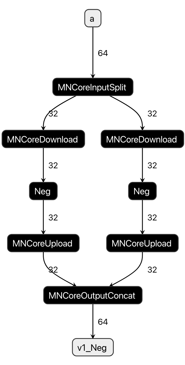
Fig. 6.3 Time-Slice for a and Neg
6.3.6. Node Simulation
For each MNNode, we estimate the memory usage and execution time when Code Emit is performed under multiple configurations.
These results are reused by enabling the enable_codegen_cache setting in mlsdk.CacheOptions.
Settings that may change during Node Simulation include:
Location (LM0 / LM1 or whether to update inputs/outputs in-place)
Whether discarded input MNValues can be safely removed after Code Emit
Configuration options available for some operations (to select implementation variations)
6.3.7. Scheduler
The Scheduler performs the following functions:
Determines the execution order of operations based on the computation graph
Adds instructions for values on the LM (data transfers between DRAM, MNValue Forget operations, and data transfers between LM0/LM1) to enable model computation within the LM’s capacity
Specifies which operations should be recomputed if necessary
Recomputation is a technique to reduce memory usage and data transfer costs (between LM and DRAM) by increasing computational cost, which is particularly effective for the MN-Core architecture where SRAM capacity is limited and data transfer costs between LM and DRAM are significant.
6.3.8. Code Emit
The codegen Code Emitter generates assembly code by referencing information configured in the MNGraph, following these steps:
Compile each MNNode individually
Link the individual compilation results into a single assembly code
The second step involves either the Concat strategy or Merge strategy, with the latter being used depending on optimization options.
6.3.8.1. Concat
Since the Address Planner ensures address consistency across all MNNodes/MNValues, the linking process is completed by simply concatenating the compilation results for each MNNode.
6.3.8.2. L1Merge
L1Merge is one of the components in codegen that can merge two instruction sequences into a single sequence. For example, if there are instruction sequences with heavy DRAM-LM communication and those with intensive computation operations, each requiring different resources, merging them can potentially reduce the instruction sequence length.
By repeatedly applying L1Merge to each compilation result, it essentially consolidates them into a single assembly code. However, there are some cases where it cannot be applied, such as when inputs/outputs are in-place, in which case additional processing like address reordering (MNCoreReorderAddress) becomes necessary.
6.3.9. GPFNApp
GPFNApp refers to an object that packages assembly code (VSM) along with the necessary execution data using flatbuffers.
It can be regarded as the compilation result from codegen. In MLSDK, it is loaded and prepared for execution within mlsdk.Context.compile().
It is also saved when mlsdk.CacheOptions are configured.
The contents are primarily divided into the following categories:
The /opt/pfn/pfcomp/codegen/build/integration/dump_gpfnapp tool included with MLSDK can be used to inspect the contents of GPFNApp in the codegen_dir.
VSM: Pre-compiled assembly code. Also referred to as GPFNBin.
Information about input/output nodes: Includes name, Dtype, Layout, Address, etc.
Parameters from the original model used for compilation
Information for relocating GPFNBin (relocation info)
Some fields are currently not supported by MLSDK.