3. Migration Tutorial
This document outlines the process for integrating MLSDK into your PyTorch application and migrating to the MN-Core series.
3.1. Migration Process
When migrating your code, it’s crucial to incrementally expand functionality on MN-Core 2 in a step-by-step manner. For example, if you have a model already running on a GPU or another backend, you should begin by migrating the inference process using your trained model, verifying its operation before proceeding with the training process.
Here, we’ll examine a specific migration workflow using the MNCoreClassifier model, as introduced in Machine Learning Tutorial.
48class MNCoreClassifier(torch.nn.Module):
49    def __init__(self):
50        super().__init__()
51        self.linear1 = torch.nn.Linear(1024, 256)
52        self.linear2 = torch.nn.Linear(256, 10)
53
54    def forward(self, x, t, **args):
55        x_reshaped = x.reshape(x.size(0), -1)
56        x1 = self.linear1(x_reshaped)
57        x2 = torch.nn.functional.relu(x1)
58        y = self.linear2(x2)
59        loss = torch.nn.functional.cross_entropy(y, t)
60        if self.training:
61            return {"loss": loss}
62        else:
63            return {"y": y, "loss": loss}
The mnist.py script located in the /opt/pfn/pfcomp/codegen/examples/ directory runs both training and inference for the MNCoreClassifier model on MN-Core 2. The corresponding PyTorch-only implementations for these processes are the mnist_train.py and mnist_infer.py scripts.
We’ll proceed with the following sequence:
Verify the operation of the original migration source program
Test execution with
pfvm:cpuTest execution with
mncore2:auto
3.1.1. Inference Process
16def main(checkpoint_path: str, outdir: str, option_json_path: Optional[Path], device_str: str) -> None:
17    batch_size = 64
18    eval_batch_size = 125
19
20    _, eval_loader = mnist_loaders(batch_size, eval_batch_size)
21
22    checkpoint = torch.load(checkpoint_path)
23
24    model_with_loss_fn = MNCoreClassifier()
25    model_with_loss_fn.load_state_dict(checkpoint["model_state_dict"])
26    model_with_loss_fn.eval()
27
28    def eval_step(inp: Mapping[str, torch.Tensor]) -> Mapping[str, torch.Tensor]:
29        x = inp["x"]
30        t = inp["t"]
31        output = model_with_loss_fn(x, t)
32        y = output["y"]
33        _, predicted = torch.max(y, 1)
34        correct = (predicted == t).sum()
35        return {"correct": correct}
36
37    correct = 0
38    for sample in eval_loader:
39        correct += eval_step(sample)["correct"]
40    print(
41        f"Correct: {correct} / {len(eval_loader.dataset)}. "
42        f"Accuracy: {correct / len(eval_loader.dataset)}"
43    )
44    assert 0.95 < correct / len(eval_loader.dataset)
Verifying the mnist_infer.py Implementation
First, ensure the inference process runs correctly in PyTorch by following the instructions in Example: Inference MNIST. Your trained checkpoint should be saved at /tmp/mlsdk_mnist/checkpoint.pt if you have already executed Example: MNIST on MN-Core 2.
Your verification is complete when the output matches the inference results obtained during training.
Testing with pfvm:cpu
Next, modify the mnist.py script to compile and call the eval_step function, as demonstrated in this example.
Upon executing the modified script, specify --device as pfvm:cpu to use the PFVM runtime for processing.
Additionally, you can pass compilation options via --option_json. Below is an example JSON configuration that instructs the compiler to generate Compiled ONNX output. For unmodified mnist.py, the <codegen_dir> should default to /tmp/mlsdk_mnist_infer/eval_step.
{
    "args": [
        "--out_onnx=<codegen_dir>/pfvm.onnx"
    ]
}
If execution completes successfully, you should find two ONNX files in the codegen_dir directory: model.onnx (Exported ONNX) and pfvm.onnx (Compiled ONNX). These ONNX files can be visualized using Netron, which is integrated into the Codegen Dashboard.
If the execution terminates abnormally, please refer to the differences between mnist.py and Common Errors and Solutions for troubleshooting.
If the execution completes normally but produces abnormal results, trying these model visualizations can help identify discrepancies in the processing steps.
First, let’s examine Fig. 3.1, which visualizes the model.onnx file.
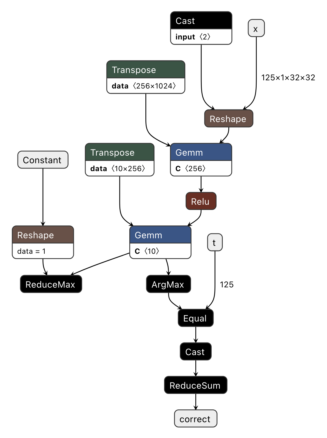
Fig. 3.1 Visualizing model.onnx (Exported ONNX)
This visualization clearly shows that eval_step’s input/output variables (x, t, correct) correspond to the ONNX’s input/output parameters. Additionally, we observe that the output of Transpose serves as the right input for Gemm, while the unused branch of torch.max (ReduceMax) remains intact.
As such, at the Exported ONNX stage, the computation graph closely mirrors the original PyTorch operations.
The PFVM-compiled version of this computation graph is pfvm.onnx, which we will now examine in Fig. 3.2.
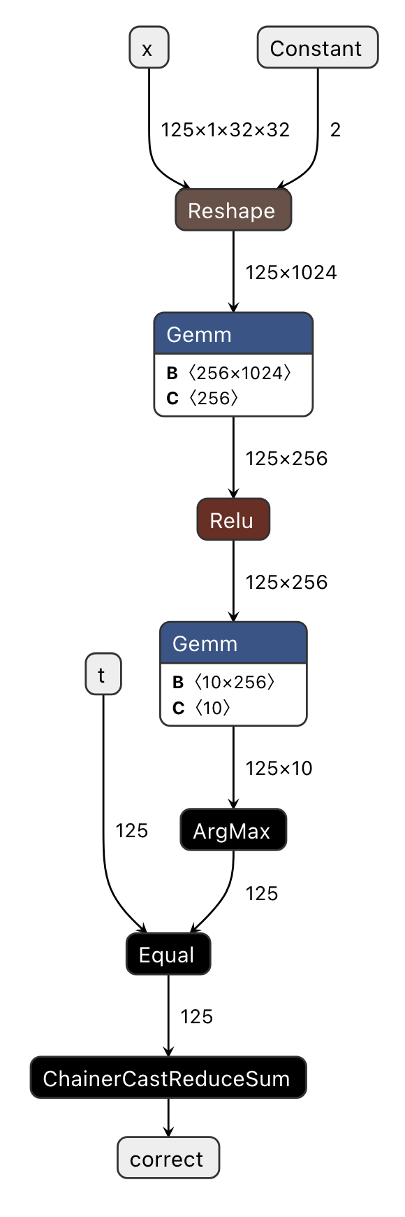
Fig. 3.2 Visualizing pfvm.onnx (Compiled ONNX)
The original computation graph has undergone several optimizations, resulting in a streamlined graph. This optimization enables significant advantages in terms of both memory usage and execution speed when utilizing the PFVM backend with GPUs (pfvm:cuda), rather than CPUs or MN-Core 2 processors, compared to the original PyTorch implementation.
Constantization of the
shapeinput parameter inReshapeOperator Fusion
Eliminates the
Transposeoperation on the right input ofGemmby settingtransB=1Consolidates consecutive
CastandReduceSumoperations into a singleChainerCastReduceSumoperator
Eliminates redundant operations surrounding
ReduceMaxwhen the result is not used
Note
Many of PFVM’s custom ONNX operators have name prefixes of MNCore or Chainer.
By comparing this graph with the implementation of eval_step and verifying any potential discrepancies in how ONNX handles these operations, we have successfully achieved our visualization objectives.
Verification with mncore2:auto
Finally, let’s verify that eval_step functions correctly by specifying mncore2:auto as the device via the --device option.
If the execution completes successfully, you should find l3ir_stripped.onnx.zst in the codegen_dir directory.
Decompress this file (using zstd -d) and visualize it in codegen-dashboard to compare with Fig. 3.3.
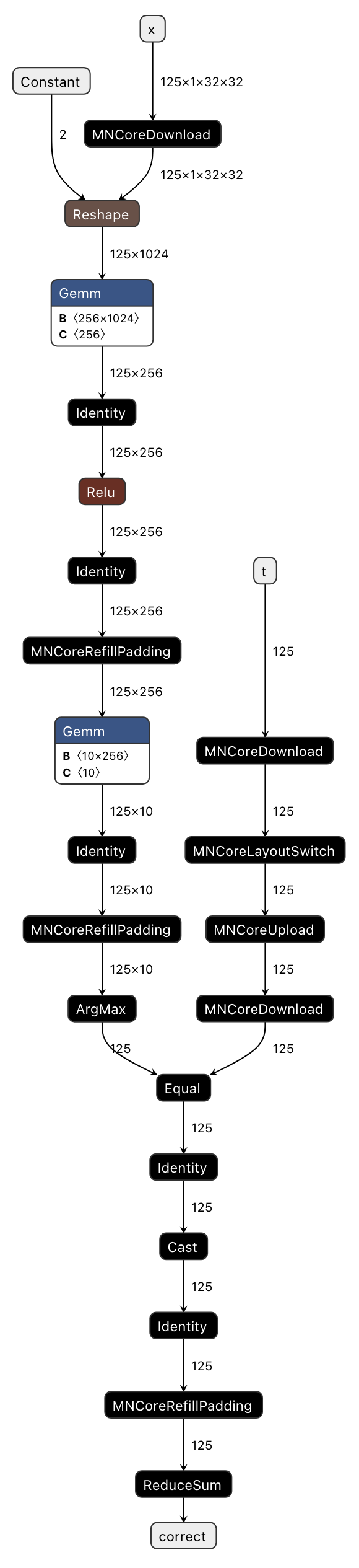
Fig. 3.3 Visualizing l3ir_stripped.onnx (MNGraph)
Comparing with Fig. 3.2, we can see that l3ir_stripped.onnx essentially represents pfvm.onnx with additional custom operators.
List of custom operators added in this example:
MNCoreUpload/MNCoreDownload: Transfers MNValue between LM → DRAM (Upload) or DRAM → LM (Download) directionsMNCoreLayoutSwitch: Converts the layout of MNValueIdentity: Moves MNValue to the opposite LM (there are two types: LM0 and LM1)MNCoreRefillPadding: Writes values (e.g., kZero, kInf) into padding areas within the layout
Additionally, MNGraph contains information about which operators to execute in what order.
This information is consolidated in l3ir.txt within codegen_dir, and for this example it contains the following content:
Constant() -> (val_1_fx2onnx)
  out(0):val_1_fx2onnx onnx_type=Tensor(dtype=INT64 shape=2) num_lw=2 padded_shape=8 layout=PadLayout{(2)/((8_L1B:1); B@[PE,W,MAB,L2B])} layout_kind=MNCore dtype=Int gene=[] loc_kind=IMM loc=IMM)
MNCoreDownload(t) -> (t_Download_1)
   in(0):t onnx_type=Tensor(dtype=INT64 shape=125) num_lw=2 padded_shape=128 layout=PadLayout{(125)/((8_L2B:1, 8_L1B:1, 1:1, 2_W:1); B@[PE,MAB])} layout_kind=MNCore dtype=Int gene=[Nr] loc=DRAM addr=0)
  out(0):t_Download_1 onnx_type=Tensor(dtype=INT64 shape=125) num_lw=2 padded_shape=128 layout=PadLayout{(125)/((8_L2B:1, 8_L1B:1, 1:1, 2_W:1); B@[PE,MAB])} layout_kind=MNCore dtype=Int gene=[Nr] loc=LM0 addr=0)
MNCoreLayoutSwitch(t_Download_1) -> (t_LayoutSwitch_0)
   in(0):t_Download_1 onnx_type=Tensor(dtype=INT64 shape=125) num_lw=2 padded_shape=128 layout=PadLayout{(125)/((8_L2B:1, 8_L1B:1, 1:1, 2_W:1); B@[PE,MAB])} layout_kind=MNCore dtype=Int gene=[Nr] loc_kind=LM loc=LM0 addr=0)
  out(0):t_LayoutSwitch_0 onnx_type=Tensor(dtype=INT64 shape=125) num_lw=2 padded_shape=128 layout=PadLayout{(125)/((8_L2B:1, 8_L1B:1, 2:1); B@[PE,W,MAB])} layout_kind=MNCore dtype=Int gene=[Nr] pad_type=Dirty loc_kind=LM loc=LM0 addr=4)
MNCoreUpload(t_LayoutSwitch_0) -> (t_LayoutSwitch_0_Upload_0)
   in(0):t_LayoutSwitch_0 onnx_type=Tensor(dtype=INT64 shape=125) num_lw=2 padded_shape=128 layout=PadLayout{(125)/((8_L2B:1, 8_L1B:1, 2:1); B@[PE,W,MAB])} layout_kind=MNCore dtype=Int gene=[Nr] pad_type=Dirty loc=LM0 addr=4)
  out(0):t_LayoutSwitch_0_Upload_0 onnx_type=Tensor(dtype=INT64 shape=125) num_lw=2 padded_shape=128 layout=PadLayout{(125)/((8_L2B:1, 8_L1B:1, 2:1); B@[PE,W,MAB])} layout_kind=MNCore dtype=Int gene=[Nr] pad_type=Dirty loc=DRAM addr=526869888)
MNCoreDownload(x) -> (x_Download_0)
   in(0):x onnx_type=Tensor(dtype=FLOAT32 shape=125,1,32,32) num_lw=8 padded_shape=128,1,32,32 layout=PadLayout{(125,1,32,32)/((8_L2B:1, 8_L1B:1, 2:1), (), (16_MAB:1, 2:4), (2:2, 4_W:1, 4_PE:1))} layout_kind=MNCore dtype=Half gene=[N,,,] pad_type=Zero loc=DRAM addr=1024)
  out(0):x_Download_0 onnx_type=Tensor(dtype=FLOAT32 shape=125,1,32,32) num_lw=8 padded_shape=128,1,32,32 layout=PadLayout{(125,1,32,32)/((8_L2B:1, 8_L1B:1, 2:1), (), (16_MAB:1, 2:4), (2:2, 4_W:1, 4_PE:1))} layout_kind=MNCore dtype=Half gene=[N,,,] pad_type=Zero loc=LM0 addr=0)
Reshape(x_Download_0, val_1_fx2onnx) -> (view_fx2onnx)
   in(0):x_Download_0 onnx_type=Tensor(dtype=FLOAT32 shape=125,1,32,32) num_lw=8 padded_shape=128,1,32,32 layout=PadLayout{(125,1,32,32)/((8_L2B:1, 8_L1B:1, 2:1), (), (16_MAB:1, 2:4), (2:2, 4_W:1, 4_PE:1))} layout_kind=MNCore dtype=Half gene=[N,,,] pad_type=Zero loc_kind=LM loc=LM0 addr=0)
   in(1):val_1_fx2onnx onnx_type=Tensor(dtype=INT64 shape=2) num_lw=2 padded_shape=8 layout=PadLayout{(2)/((8_L1B:1); B@[PE,W,MAB,L2B])} layout_kind=MNCore dtype=Int gene=[] loc_kind=IMM loc=IMM)
  out(0):view_fx2onnx onnx_type=Tensor(dtype=FLOAT32 shape=125,1024) num_lw=8 padded_shape=128,1024 layout=PadLayout{(125,1024)/((8_L2B:1, 8_L1B:1, 2:1), (16_MAB:1, 4:2, 4_W:1, 4_PE:1))} layout_kind=MNCore dtype=Half gene=[N,C] pad_type=Zero loc_kind=LM loc=LM0 addr=0 parent=x_Download_0)
Gemm(view_fx2onnx, attr_0, attr_1, transB) -> (addmm_fx2onnx)
   in(0):view_fx2onnx onnx_type=Tensor(dtype=FLOAT32 shape=125,1024) num_lw=8 padded_shape=128,1024 layout=PadLayout{(125,1024)/((8_L2B:1, 8_L1B:1, 2:1), (16_MAB:1, 4:2, 4_W:1, 4_PE:1))} layout_kind=MNCore dtype=Half gene=[N,C] pad_type=Zero loc_kind=LM loc=LM0 addr=0 parent=x_Download_0)
   in(1):attr_0 onnx_type=Tensor(dtype=FLOAT32 shape=256,1024) num_lw=1024 padded_shape=256,1024 layout=PadLayout{(256,1024)/((16:64, 4_W:1, 4_PE:1), (16_MAB:1, 4:16, 4:1, 4:4); B@[L1B,L2B])} layout_kind=MNCore dtype=Half gene=[WC,WC] loc_kind=DRAM loc=DRAM addr=9216)
   in(2):attr_1 onnx_type=Tensor(dtype=FLOAT32 shape=256) num_lw=2 padded_shape=256 layout=PadLayout{(256)/((16_MAB:1, 2:1, 2_W:1, 4_PE:1); B@[L1B,L2B])} layout_kind=MNCore dtype=Float gene=[WC] loc_kind=DRAM loc=DRAM addr=25600)
  out(0):addmm_fx2onnx onnx_type=Tensor(dtype=FLOAT32 shape=125,256) num_lw=2 padded_shape=128,256 layout=PadLayout{(125,256)/((8_L2B:1, 8_L1B:1, 2:1), (16_MAB:1, 4_W:1, 4_PE:1))} layout_kind=MNCore dtype=Half gene=[N,C] pad_type=Dirty loc_kind=LM loc=LM1 addr=0)
...
Due to the limitations of space, we cannot reproduce the entire contents of l3ir.txt. Here we explain each operator based on the provided snippet.
By the way, in MNGraph, each operator is referred to as MNNode, and its inputs and outputs are called MNValue.
For example, in the notation Constant() -> (val_1_fx2onnx), Constant represents the MNNode and val_1_fx2onnx represents the MNValue.
Additionally, in(...): and out(...): provide detailed descriptions of the corresponding MNValue.
Constant() -> (val_1_fx2onnx): Creates a constant tensor to be input to theReshapeoperator. SinceConstanthas no dependencies, it is typically scheduled first.MNCoreDownload(t) -> (t_Download_1): Moves input tensortfrom DRAM to LMMNCoreLayoutSwitch(t_Download_1) -> (t_LayoutSwitch_0): Changes the layout of tensortMNCoreUpload(t_LayoutSwitch_0) -> (t_LayoutSwitch_0_Upload_0): Moves the reformatted tensortback to DRAMMNCoreDownload(x) -> (x_Download_0): Moves input tensorxfrom DRAM to LMReshape(x_Download_0, val_1_fx2onnx) -> (view_fx2onnx): Reshapes tensorxGemm(view_fx2onnx, attr_0, attr_1, transB) -> (addmm_fx2onnx): Performs matrix multiplication using the newly reshaped tensorxas input
Beyond what can be explained here, the l3ir.txt file is capable of representing most of MNGraph’s information.
As the number of graph nodes increases, direct visualization of ONNX becomes increasingly challenging, making the MNGraph log file crucial for verifying its correctness.
Once you’ve confirmed that execution with mncore2:auto works correctly, you can proceed to explore more advanced scheduling options.
The following JSON example demonstrates how to specify the --scheduler compilation option:
{
    "args": [
        "--scheduler=spill_opt"
    ]
}
After applying this and rerunning the process, you can verify the effects by visualizing l3ir_stripped.onnx again. However, the most direct metric can be found in the report.json file under codegen_dir, specifically the vsm_cycles value.
vsm_cycles represents the total number of cycles required to execute the entire VSM. By dividing this by core_freq (expressed in MHz) from the same report.json, you can obtain the actual execution time.
In our testing case, with core_freq set to 750.0 MHz, the default scheduler (reuse_consecutive) resulted in 7500 cycles (0.010 msec, 6.63 TFLOPS = 1.69%), while using the spill_opt scheduler reduced this to 6932 cycles (0.009 msec, 7.17 TFLOPS = 1.82%). Although the MNCoreClassifier inference process itself has a relatively small flops value of 66,273,875 according to report.json, this still doesn’t fully leverage the MN-Core 2’s performance.
In practical scenarios, however, we can expect significantly greater improvements.
For details about optimization settings such as schedulers, please refer to Compile Options and Preset Options.
3.1.2. Training Process
18def main(outdir: str, option_json_path: Optional[Path], device_str: str) -> None:
19    batch_size = 64
20    eval_batch_size = 125
21
22    train_loader, _ = mnist_loaders(batch_size, eval_batch_size)
23
24    model_with_loss_fn = MNCoreClassifier()
25    model_with_loss_fn.train()
26
27    optimizer = torch.optim.SGD(model_with_loss_fn.parameters(), 0.1, 0.9, 0.0)
28
29    def train_step(inp: Mapping[str, torch.Tensor]) -> Mapping[str, torch.Tensor]:
30        x = inp["x"]
31        t = inp["t"]
32        optimizer.zero_grad()
33        output = model_with_loss_fn(x, t)
34        loss = output["loss"]
35        loss.backward()
36        optimizer.step()
37        return {"loss": loss}
38
39    for epoch in range(10):
40        loss = 0.0
41        for i, sample in enumerate(train_loader):
42            curr_loss = train_step(sample)["loss"]
43            loss += (curr_loss - loss) / (i + 1)
44            if i % 100 == 0:
45                print(f"epoch {epoch}, iter {i:4}, loss {loss}")
46        print(f"epoch {epoch}, loss {loss}")
47
48    os.makedirs(outdir, exist_ok=True)
49    torch.save(
50        {
51            "model_state_dict": model_with_loss_fn.state_dict(),
52            "optim_state_dict": optimizer.state_dict(),
53        },
54        storage.path(outdir) / "checkpoint.pt",
55    )
Verifying mnist_train.py Operation
First, verify that the training process runs correctly in PyTorch by referring to Example: Training MNIST. The training results will be saved in <outdir>/checkpoint.pt, allowing you to verify the results using mnist_infer.py.
If the Accuracy value exceeds 0.95, the operation verification is complete.
Testing on pfvm:cpu
Next, modify mnist.py to compile and call the train_step function, similar to Inference Process.
Specify --device as pfvm:cpu and also configure the compilation option --out_onnx.
If the execution completes successfully, you should find an ONNX file corresponding to Compiled ONNX in the codegen_dir directory.
The visualized version Fig. 3.4 appears as follows (the relationship with Exported ONNX has already been explained above, so we omit further explanation here).
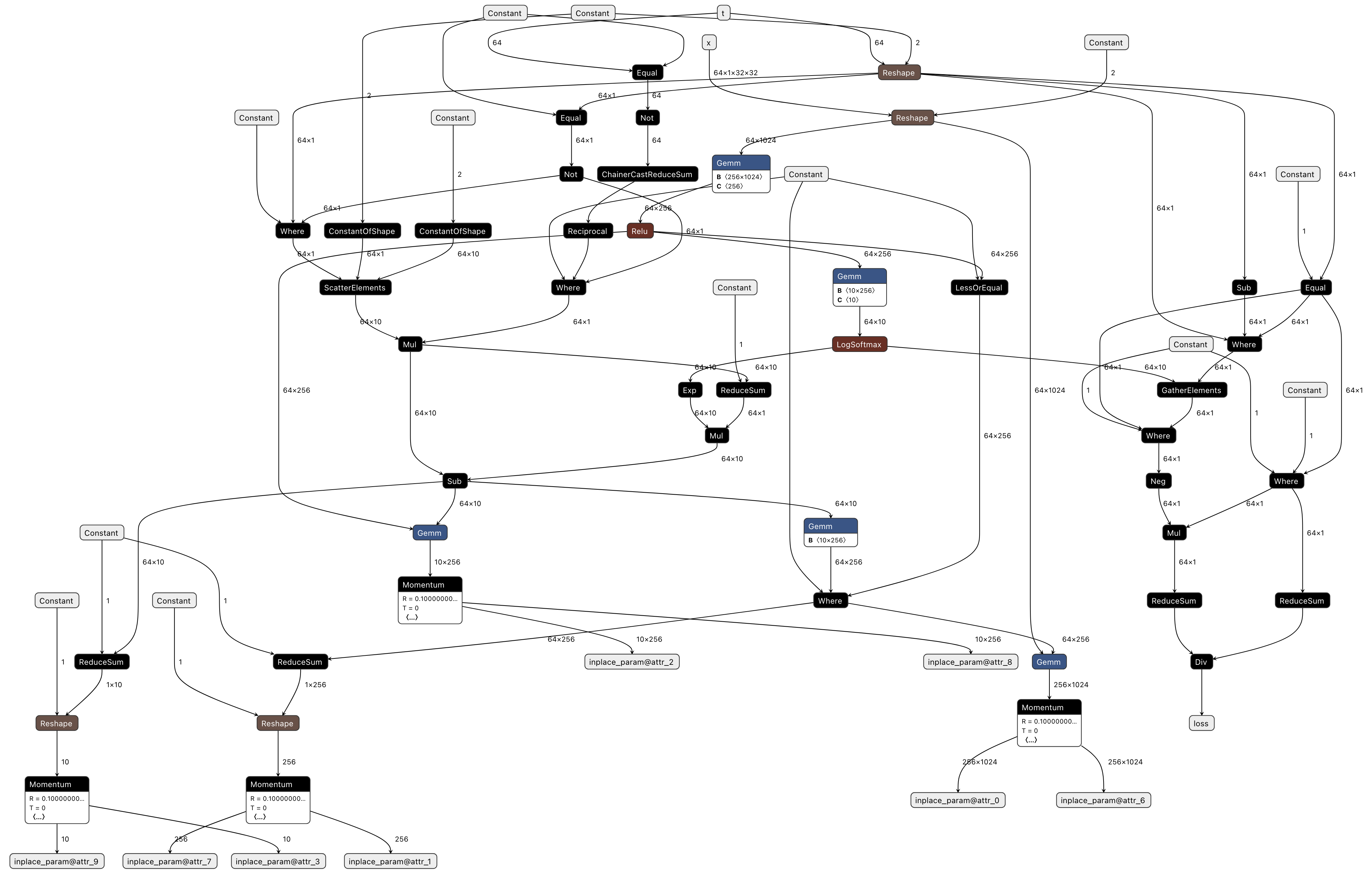
Fig. 3.4 Visualizing pfvm.onnx (Compiled ONNX)
Compared to standalone inference processing that only performs forward passes, the graph becomes significantly larger when backward propagation and optimizer processing are added. Additionally, backward propagation and optimizer processing often aren’t included in the original program implementation, making it difficult to properly map each node. Therefore, we recommend first verifying that the forward processing works correctly before adding backward and optimizer processing.
Now, even when training appears to complete normally and the loss decreases, upon examining the training checkpoint, you may find that the Accuracy hasn’t improved sufficiently. In such cases, the issue might be that the model or optimizer’s internal torch.Tensor objects aren’t registered in the Context, and changes made on the device aren’t being reflected even after calling Context.synchronize.
Details about this mechanism are also explained in Registering Parameters with the Context and Registering Optimizer Buffers with the Context.
Verification with mncore2:auto
Finally, let’s verify whether the train_step function runs on MN-Core 2 by specifying the --device option as mncore2:auto.
The final Accuracy may differ from that obtained with pfvm:cpu, but this is because the implementations of individual operators differ—provided the numerical results are above the acceptable threshold, this difference is acceptable.
While the MNCoreClassifier itself isn’t particularly large as a model, the number of operators within the MNGraph easily exceeds 100, making it difficult to visualize the ONNX representation and properly map it to the original implementation. For examining the contents of the MNGraph, we recommend checking the l3ir.txt file instead.
3.2. Advanced Topics
Advanced Features describes features not covered in
add.pyandmnist.pySample programs utilizing the MLSDK can be found from the Gallery