4. Advanced Features
4.1. Features of gpfn3-smi
As a general principle of the MLSDK, users should not need to use any gpfn3-smi commands except list.
Device initialization processes are primarily handled automatically.
However, there may be cases where devices malfunction due to unintended reasons, or when advanced debugging is required, so we will also introduce these commands here.
For details about various commands and their usage, you can also check by specifying the --help option, but we recommend not using any commands beyond those described here.
4.1.1. gpfn3-smi list
Displays a list of available devices.
0: mnc2p27s0
1: mnc2p28s0
2: mnc2p42s0
3: mnc2p43s0
4: mnc2p171s0
5: mnc2p172s0
6: mnc2p187s0
7: mnc2p188s0
Device information is displayed in the format (Device Index): (Device Name).
The Device Index is a 0-based sequential number assigned to each available device, while the Device Name represents the name of the device on the compute node.
Since the available devices may change due to PFCP-side mechanisms, the mapping between Device Index and Device Name is not fixed.
When specifying which device to use for mlsdk.MNDevice, you should provide either the Device Index or auto.
4.1.2. gpfn3-smi reset <device>
Issues a reset to the specified device.
Usage: gpfn3-smi reset [options...] <device>

Examples:
    gpfn3-smi reset 0
<device> can accept either a Device Index or Device Name.
If executed successfully, the reset for the specified device will be completed.
Warning
If you reset a device that is currently locked by another program, progress made by that program may be lost.
4.1.3. gpfn3-smi clear <device>
Initializes all memory on the specified device (including DRAM, registers, etc.) with the specified value.
Clears all memory on the device. Mask registers are set to all ones regardless of the options.

Usage: gpfn3-smi clear [options...] <device>

Options:
  -pattern uint
         Fills the memory with the specified uint64 value instead of random bytes
  -seed int
         Seed value for random byte generation
  -zero
         Fills the memory with zeros instead of random bytes

Examples:
    gpfn3-smi clear --seed 1234 0
    gpfn3-smi clear --zero 0
    gpfn3-smi clear --pattern 0x5555555555555555 0
Due to the large amount of memory initialization involved, execution may take considerable time to complete.
4.2. Compile Options
The options parameter in mlsdk.Context.compile() primarily includes Compile Options that primarily affect the behavior of the code generator.
For example, when specifying both option_json and float_dtype, the configuration would look like this:
context.compile(
    ...
    options={
        "option_json": "/opt/pfn/pfcomp/codegen/preset_options/O1.json",
        "float_dtype": "float",
    },
)
Compile Options can be specified either as command-line options or as environment variables.
Through options, you primarily specify the former, but option_json also allows you to specify the latter.
Below we describe the available items for Compile Options.
4.2.1. Preset Options
A collection of preconfigured settings that combine appropriate options from the Compile Options menu to suit different user scenarios.
In MLSDK environments, these Preset Options are located under /opt/pfn/pfcomp/codegen/preset_options/.
O0.json: Prioritizes successful code generation compilation.O1.json: Uses the same scheduler as O2 and later, but with the most conservative optimization settings.O2.json: Implements scheduling utilizing simulated annealing.O3.json: Expands the search space from O2 and incorporates L1Merge.O4.json: Further expands the search space from O3.debug.json: Uses a simple scheduler without complex optimizations.
The optimization level increases from O0 to O4, resulting in higher final performance, but at the cost of longer scheduling times.
Especially for O2 and later versions, the time spent on Node Simulation and subsequent simulated annealing increases, so we recommend using O1 or lower for basic compilation verification.
We also recommend reusing the results of Node Simulation by setting mlsdk.CacheOptions.
For “debug”, the configuration minimizes optimizations to facilitate easier examination of compilation results, making it less reliable for actual use compared to O0 or O1. Therefore, it isn’t intended for regular production use.
4.2.2. Command Line Options
4.2.2.1. option_json
Accepts the path to a JSON file containing compilation options, including environment variables. The JSON format is as follows:
{
    "envs": {
        "<CODEGEN_ENV_NAME>": <CODEGEN_ENV_VALUE>,
        ...
    },
    "args": [
        "--<option_name>=<option_value>",
        ...
    ],
    "name": <name>
}
envs: Allows specification of valid environment variables. If an existing environment variable is specified, the value inoption_jsonwill be ignored.args: Specifies each option in the order they appear. For example, to specifyfloat_dtype, use"--float_dtype=float". This option is ignored ifoption_jsonis specified (nested specifications are not supported).name(optional) : Allows assigning a name to the configuration.
Additionally, the option.json file generated in codegen_dir is a JSON file that can be specified in option_json.
By respecifying this file, you can reproduce the exact compilation options used when creating that codegen_dir.
4.2.2.2. float_dtype
An option that specifies which floating-point data type codegen should assign to Tensors of type torch.float32.
Also see the description for options in mlsdk.Context.compile().
options={"float_dtype": "<value>"},
mixed: Uses half-precision for GEMM operations (both input and output), and float precision otherwisehalf: Assigns half-precision to all such tensorsfloat: Assigns float precision to all such tensorsdouble: Assigns double-precision to all such tensors
4.2.2.3. layout_planner
Configures the Layout Planner.
options={"layout_planner": "<value>"},
lpz: Uses Layout Planner Zbidi: Uses bidirectional layout plannerlegacy: Uses legacy layout planner
4.2.2.4. scheduler
Configures the Scheduler.
options={"scheduler": "<value>"},
always_from_dram: Always downloads data from DRAM before executing each operation and uploads the outputs after execution.reuse_consecutive: Similar toalways_from_dram, but utilizes existing data in SRAM output by the previous layer.spill_opt: Delays uploading data until SRAM becomes full.auto_recompute_sa: Anneals the order of operations and SRAM-only values.
4.2.2.5. simulation_mode
Configures the Node Simulation.
options={"simulation_mode": "<value>"},
auto: Selects an appropriatesimulation_modebased on thescheduler.default: Simulates appropriate patterns of ConstrainAssignment.fast: Simulates specific patterns of ConstrainAssignment.best: Simulates all possible patterns of ConstrainAssignment, with some simulations potentially failing.full: Simulates all patterns of ConstrainAssignment regardless of any failures.fake: No actual simulation, only rough estimations. (Hence the fastest option.)
4.2.2.6. sram_budget
Specifies the percentage of available LM resources to use, ranging from 0 to 1 (default).
options={"sram_budget": <value>},
4.2.2.7. sa_expected_run_iters
Specifies the number of iterations for the annealing-based optimization loop.
options={"sa_expected_run_iters": <value>},
4.2.2.8. out_onnx
Outputs the optimized ONNX to the specified path in MLSDK Pipeline and Backend Correspondence.
options={"out_onnx": <path>},
4.2.3. Environment Variables
4.2.3.1. CODEGEN_FIND_BEST_COMPILE_OPTIONS
Try all available Emit strategies and find the optimal one.
4.2.3.2. CODEGEN_FIND_BETTER_COMPILE_OPTIONS
Try out reasonable options from the available Emit strategies and find the optimal one.
4.2.3.3. CODEGEN_SCHEDULE_PP_BEAM_MAX_TURN
Maximum number of turns in the beam search for node reordering. -1 means no limit.
4.2.3.4. CODEGEN_SCHEDULE_PP_BEAM_TURN_PRUNE_LIMIT
Maximum number of turns without improvement in the beam search for node reordering.
4.2.3.5. CODEGEN_SCHEDULE_PP_BEAM_WIDTH
Maximum number of candidates to consider in the beam search for node reordering.
4.2.3.6. CODEGEN_USE_MERGE
Enable l1merge
4.2.3.7. CODEGEN_USE_PARALLEL_MERGE
Parallelize l1merge in an O(log(N)) manner
4.3. Directly loading codegen_dir
While setting cache options allows reusing compilation results, this incurs additional overhead as function tracing is required to select the appropriate GPFNApp during reruns.
Conversely, using mlsdk.Context.load_codegen_dir() to directly reuse codegen_dir avoids this tracing overhead.
However, this assumes consistency in compiled functions and input tensor dimensions, making it unsuitable for typical development use cases.
4.3.1. Usage Example
See Example: Load codegen_dir for usage examples.
8# Load the previously compiled function
9loaded_add = context.load_codegen_dir(storage.path("/tmp/add_two_tensors"))
A mlsdk.CompiledFunction can be created directly without calling mlsdk.Context.compile().
4.4. Codegen Dashboard
The Codegen Dashboard is a tool for inspecting contents of codegen_dir in a web browser.
Note
Some files within codegen_dir are compressed using Zstandard and have the .zst extension.
Such files may not be able to be properly directed to a viewer and may require decompression first.
$ cd <codegen_dir> && zstd -d <filename>.zst
4.4.1. Starting the Dashboard
Run
codegen-dashboard-externalinservemode within the workspace Pod.
$ /opt/pfn/pfcomp/codegen/build/codegen-dashboard/codegen-dashboard-external serve <codegen_dir> --port 8327
Perform a local
kubectl port-forwardto the specified port.
$ kubectl port-forward pod/<pod-name> 8327:8327
Access
http://localhost:8327in your web browser.
4.4.2. Summary
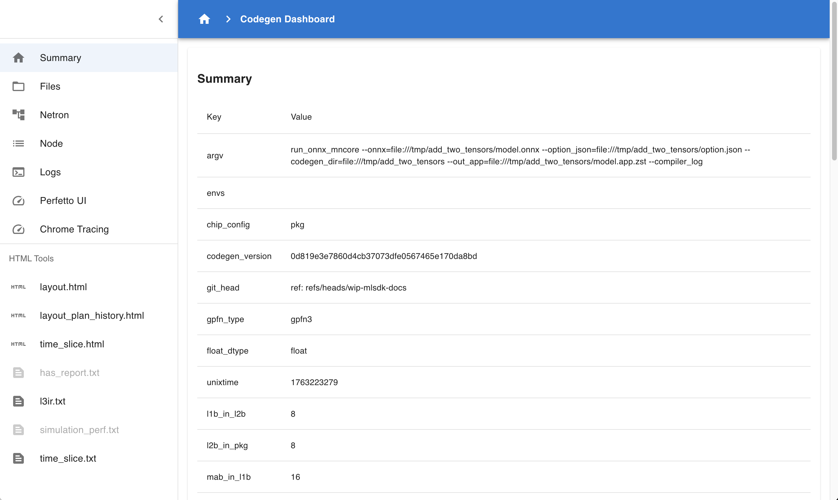
Fig. 4.1 Codegen Dashboard: Summary
This page summarizes the contents of codegen_dir.
Summary : Displays information about executed commands, hardware configuration, etc.
flopsspecifically indicates the number of computations in the computation graph, allowing rough estimation of scale.Compile Statuses : Lists whether each Phase was successful and the time taken.
Layers : Displays information about each Layer in MNGraph.
Perf Stats : Breaks down Layer contents by attribute and summarizes processing times for each.
ALLspecifically represents the total computation time, enabling verification of optimization levels achieved through Compile Options.
4.4.3. Netron
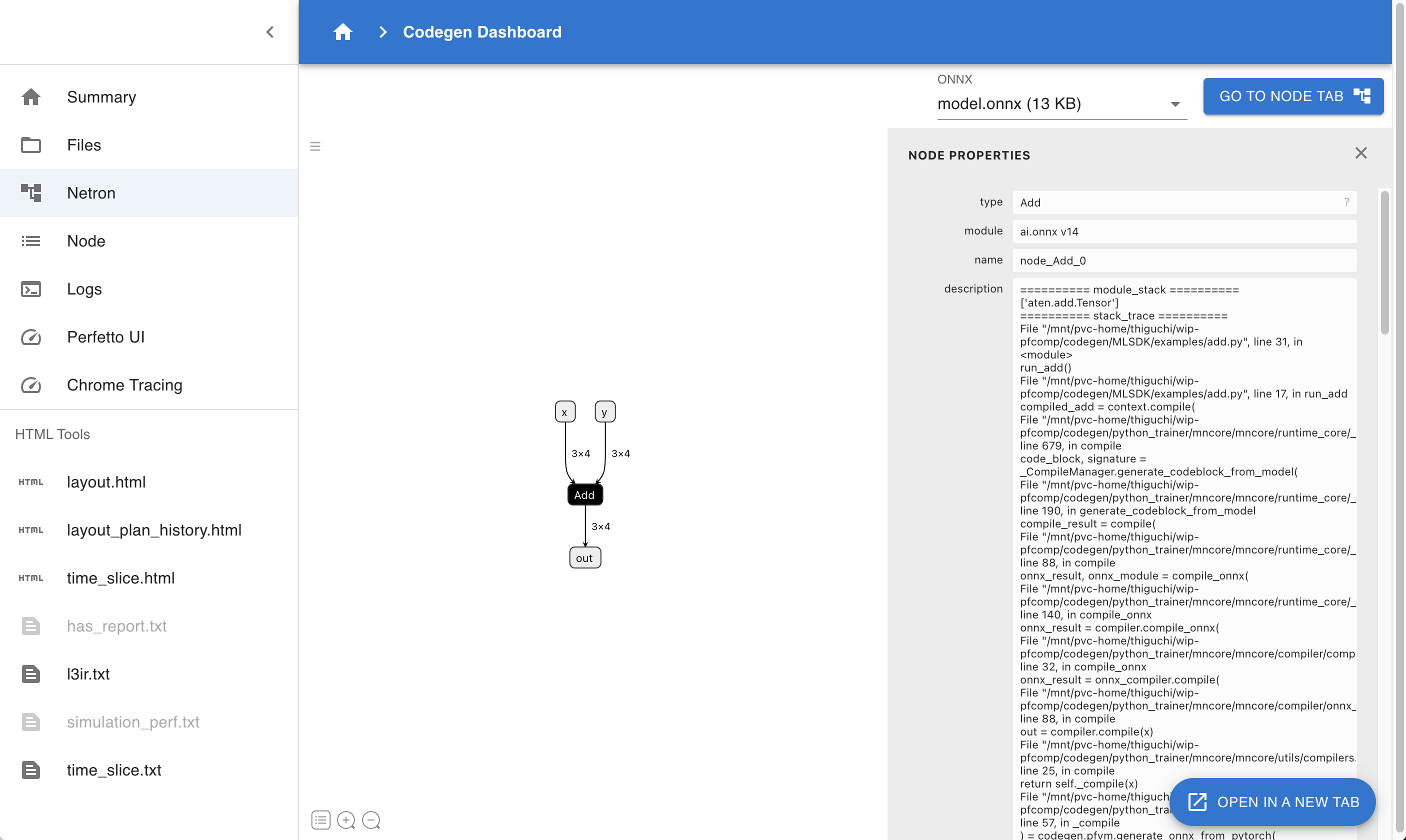
Fig. 4.2 Codegen Dashboard: Netron
Use Netron to visualize ONNX files contained in codegen_dir. If multiple ONNX files exist, you can choose which one to examine.
4.4.4. Node
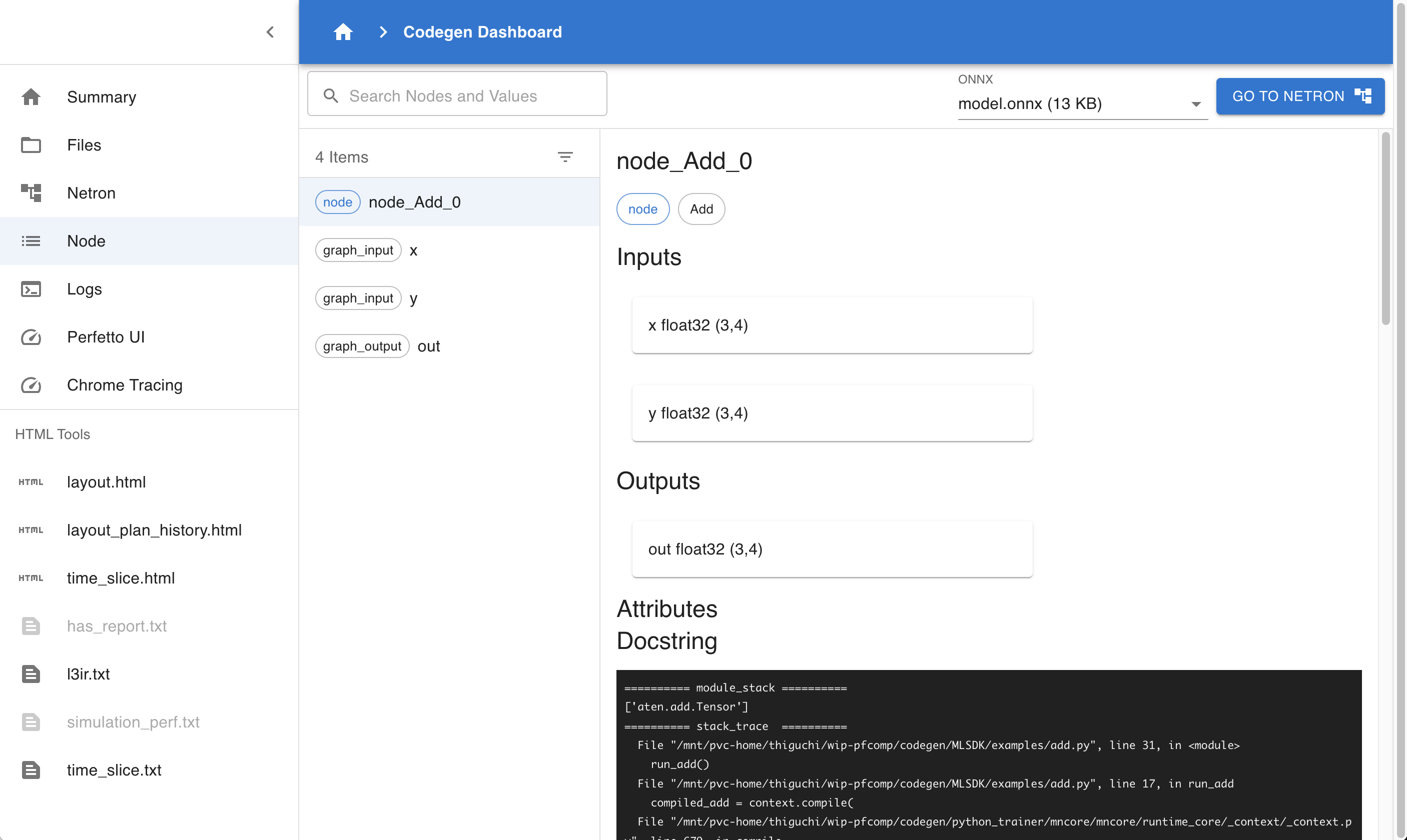
Fig. 4.3 Codegen Dashboard: Node
Similar to Netron, this page allows inspection of ONNX file contents. However, since it doesn’t perform graph visualization, it operates more efficiently even for large cases.
4.4.5. Logs
Allows viewing MLSDK log outputs.
CLOG.log: PFVM logs.glog/codegen...: codegen logs. When running in multi-process mode, each process logs to a separate file.
4.4.6. Perfetto UI
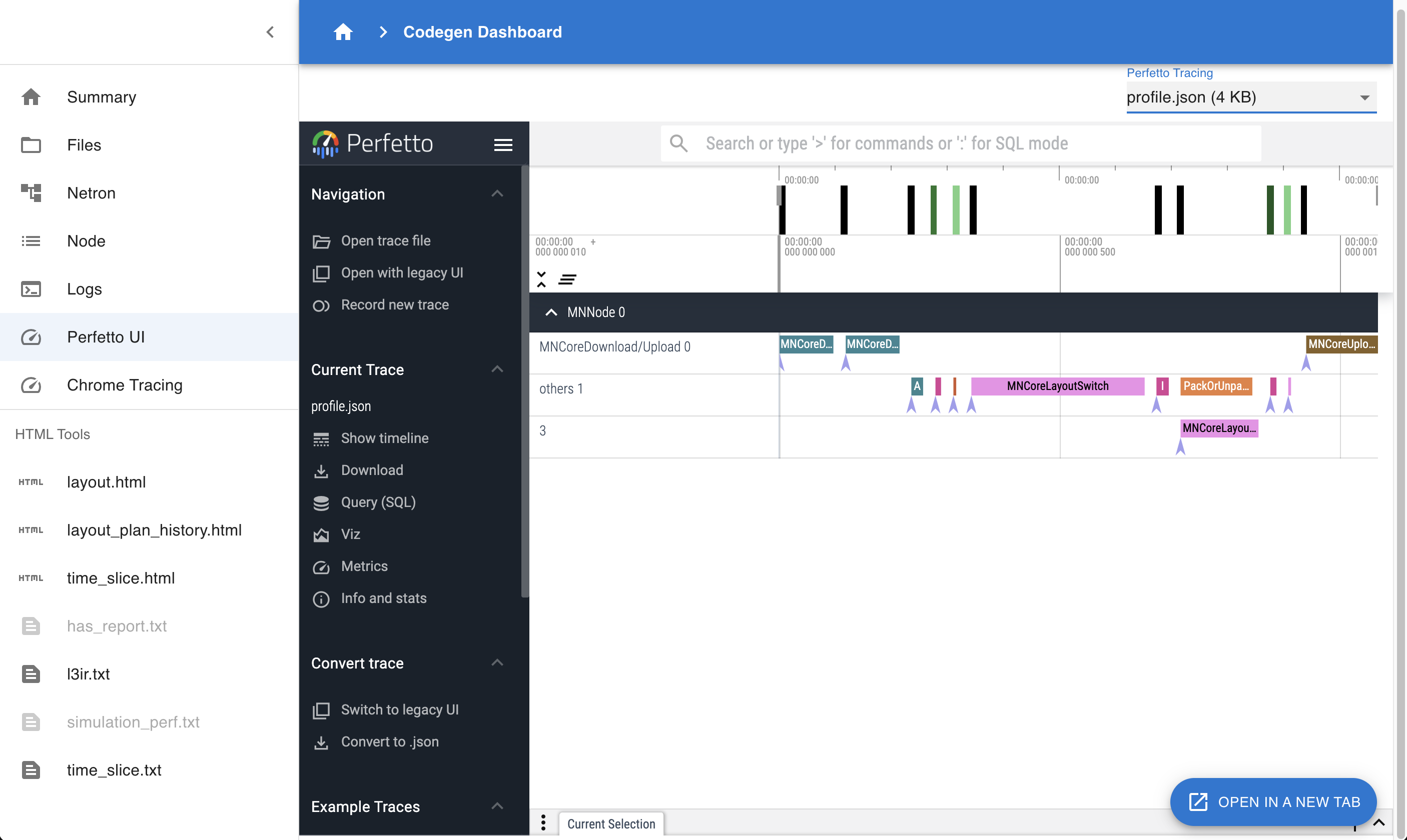
Fig. 4.4 Codegen Dashboard: Perfetto UI
Visualize Perfetto UI using files like profile.json or trace.json.
Useful for examining when each Layer executes on the device and for how long.
4.4.7. Chrome Tracing
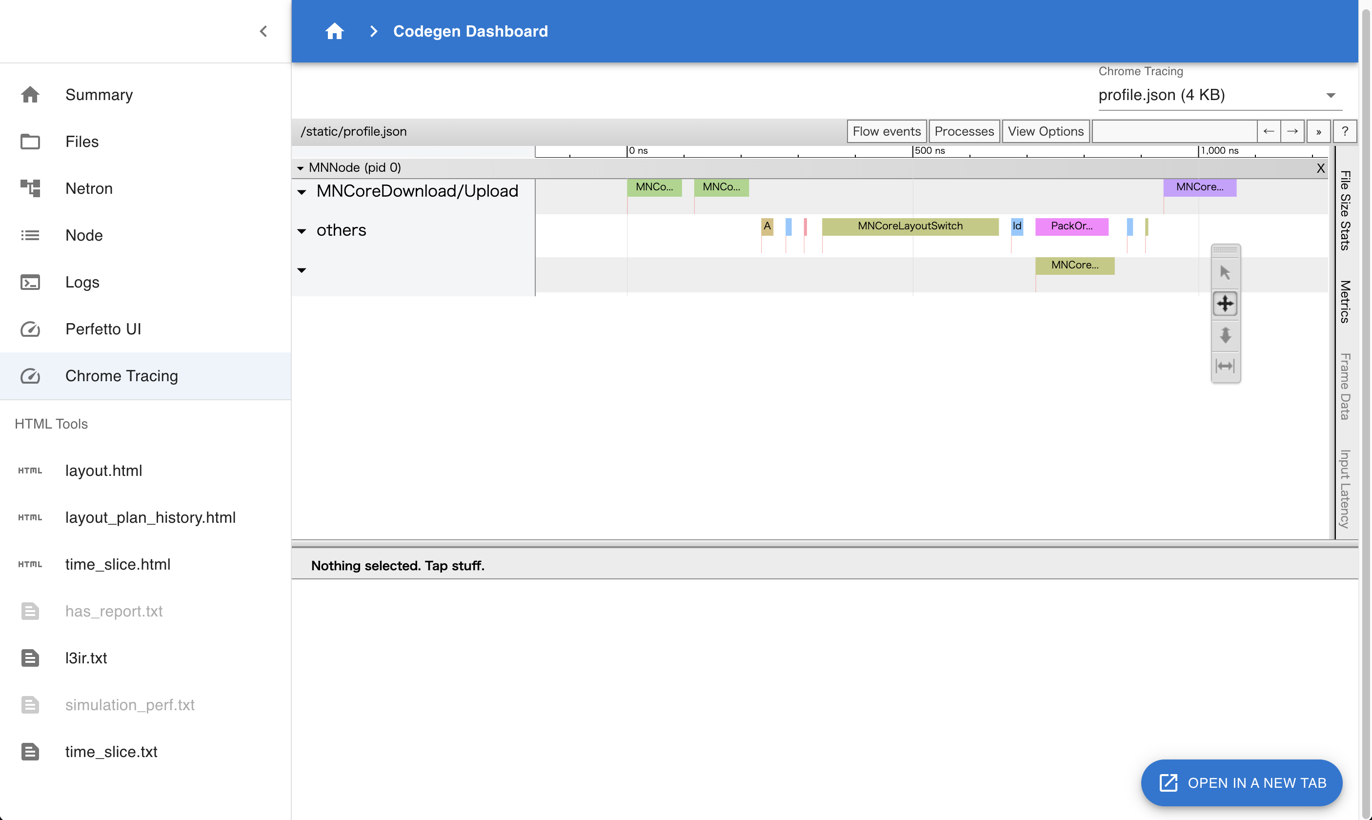
Fig. 4.5 Codegen Dashboard: Chrome Tracing
The information viewable here is essentially the same as with Perfetto UI, but this visualization uses the Chrome Tracing mechanism.
4.4.8. HTML Tools
layout.html: Contains the final Layout settings applied to the MNGraph.layout_plan_history.html: Documents the sequence of Layout configuration applied to the MNGraph.time_slice.html: Displays the Layout state immediately before graph branching occurs due to Time-Slice.l3ir.txt: Represents the MNGraph including its computation schedule.time_slice.txt: Represents the MNGraph including its computation schedule immediately before graph branching occurs due to Time-Slice.
4.5. Data Transfer via TensorProxy
mlsdk.TensorProxy is an object that represents a device-side tensor corresponding to a torch.Tensor on the host.
Examples include tensors passed as input to mlsdk.CompiledFunction or parameters registered via mlsdk.Context.register_param().
For each such case, a corresponding TensorProxy is created, and their mapping relationships are recorded in the registry within the mlsdk.Context.
Data communication between the host and device in MLSDK is handled through TensorProxy.
While device-to-host communication (D2H) requires explicit instruction by MLSDK users, as demonstrated by the mlsdk.TensorProxy.cpu() method introduced in Getting Started, host-to-device communication (H2D) occurs implicitly.
This approach generally suffices for normal usage, but for optimization purposes where you need to specify H2D timing, there are available APIs that can be used.
Note
Technically, this is an API for explicitly indicating when H2D should begin, so the entire communication process is asynchronous. Currently, we do not provide any APIs for directly checking the completion of H2D operations.
4.5.1. Obtaining TensorProxy Objects
First, you need to obtain a TensorProxy corresponding to the torch.Tensor you wish to perform H2D operations on.
Inputs for CompiledFunctions
mlsdk.CompiledFunction.allocate_input_proxy() is an API for retrieving TensorProxy objects corresponding to inputs in a CompiledFunction.
When called, it allocates a buffer on the device’s DRAM for storing the input data and returns a Dict[str, TensorProxy] object containing the corresponding keys and TensorProxy mappings.
Registered Tensors in the Context
mlsdk.Context.get_registered_value_proxy() is an API for retrieving TensorProxy objects registered with the Context using either mlsdk.Context.register_param() or mlsdk.Context.register_buffer().
In this case, since device DRAM space has already been allocated for each TensorProxy, no new DRAM allocation occurs.
The API arguments should be the torch.Tensor objects registered via register_param or register_buffer, and the corresponding TensorProxy objects will be returned.
4.5.2. Feeding Values into TensorProxy Objects
Next, you need to feed torch.Tensor values into the obtained TensorProxy objects.
mlsdk.TensorProxy.load_from() accepts a torch.Tensor object tensor and a bool flag clone, then initiates the communication process.
tensor
The value to be fed into the TensorProxy.
It can be the same object as the torch.Tensor passed to Context.compile or registered with the Context, provided the dimensions and data types match.
clone (default: True)
True: Copies the content oftensorand places it in the transfer queue. This method is safe even iftensoris modified afterward, but involves copy overhead.False: Places a reference totensorin the transfer queue. This method avoids copy costs but may result in undefined behavior iftensoris modified during transit. This is acceptable iftensoris a temporary object.
4.5.3. Usage Example
See Example: Explicitly Transferring Data Between Host And Device for usage examples.
Input for CompiledFunction
33    input_proxies_allocated = compiled_infer.allocate_input_proxy()
34    input_proxies_allocated["x"].load_from(torch.ones(4, 4), clone=False)
The prepared input_proxies_allocated is used as input for the later compiled_infer operation.
Tensors Registered in the Context
36    for model_param in model.parameters():
37        model_param_proxy = context.get_registered_value_proxy(model_param)
38        model_param_proxy.load_from(model_param)
Each model_param was originally transferred from H2D after starting compiled_infer, but we initiated the communication process beforehand.
4.5.4. Advanced Usage Tips
For use cases involving model training loops, the basic progression involves repeating these steps 1-4:
Retrieve input data from the data loader
Transfer input data from H2D
Execute the
CompiledFunctionTransfer output data from D2H (synchronous)
A key point to note is that during H2D transfers, transpose operations are required to match the MN-Core’s memory layout, making host-side processing a potential bottleneck. Therefore, interleaving steps 1 and 2 between steps 3 and 4 allows for effective overlap of host and device processing.